Chapter 5: FoSR
This book Chapter and the code in this page considers functions as responses in models with scalar predictors. This setting is widespread in applications of functional data analysis; we will focus on the linear Function-on-Scalar Regression (FoSR) model.
Motivation and Exploratory Analysis of MIMS Profiles
The code below imports and organizes data the processed NHANES data
nhanes_fda_with_r.rds and available here. This code assumes the data are
stored in the directory ./data/. We retain a small number
of scalar covariates (gender and age, as well
as the participant ID in SEQN which we convert to a factor
variable) and create a categorical age variable. Subjects who are
missing covariate information are dropped. To keep the examples in this
section computationally feasible, we use the first 250 subjects in this
dataset.
nhanes_df =
  readRDS(
    here::here("data", "nhanes_fda_with_r.rds")) %>%
  select(SEQN, gender, age, MIMS_mat = MIMS) %>%
  mutate(
    age_cat =
      cut(age, breaks = c(18, 35, 50, 65, 80),
          include.lowest = TRUE),
    SEQN = as.factor(SEQN)) %>%
  drop_na(age, age_cat) %>%
  tibble() %>%
  slice(1:250)
In the next code chunk, the MIMS variable is converted
to a tidyfun object and stored as a single column of
functional observations.
nhanes_df =
  nhanes_df %>%
  mutate(
    MIMS_tf = matrix(MIMS_mat, ncol = 1440),
    MIMS_tf = tfd(MIMS_tf, arg = seq(1/60, 24, length = 1440)))
One way to explore the associations between subject-level characteristics and 24-hour activity is to consider the MIMS profile as a response that varies according to scalar predictors like age and gender. The Figure below shows minute-level averages for participants in each age category, separately for male and female. From this, we observe a clear diurnal pattern of activity, and note a decrease in physical activity in the afternoon and evening as age increases this is particularly noticeable for male participants.
nhanes_df %>%
  group_by(age_cat, gender) %>%
  summarize(mean_mims = mean(MIMS_tf)) %>%
  ggplot(aes(y = mean_mims, color = age_cat)) +
  geom_spaghetti() +
  facet_grid(.~gender) +
  scale_x_continuous(
    breaks = seq(0, 24, length = 5),
    labels = str_c(seq(0, 24, length = 5), ":00")) +
  labs(x = "Time of day (hours)", y = "Average MIMS")
## `summarise()` has grouped output by 'age_cat'. You can override using the
## `.groups` argument.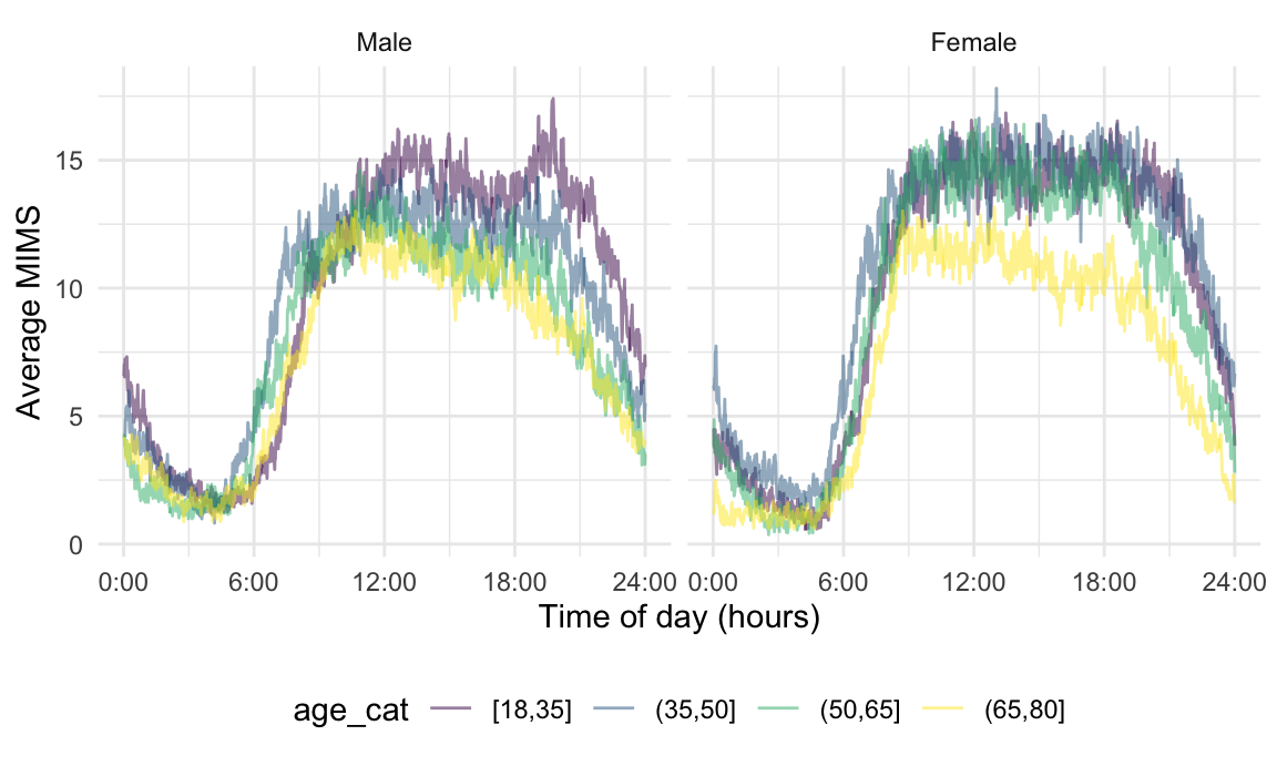
Exploratory plots like this one are useful for beginning to understand the effects of covariates on physical activity, but are limited in their scope; more formal approaches to function-on-scalar regression adjust for covariates and ensure smoothness across adjacent time points.
Regressions using Binned Data
To build intuition for functional response model interpretations, identify practical challenges, and motivate later developments, we fit a series of regressions to MIMS profiles using binned or aggregate observations. The next code chunk aggregates minute-level data into hour-length bins, so that each MIMS profile consists of 24 observations. To obtain hourly trajectories, we “smooth” minute-level data using a rolling mean with a 60-minute bandwidth and evaluate the resulting functions at the midpoint of each hour.
nhanes_df =
  nhanes_df %>%
  mutate(
    MIMS_hour =
      tf_smooth(MIMS_tf, method = "rollmean", k = 60, align = "center"),
    MIMS_hour = tfd(MIMS_hour, arg = seq(.5, 23.5, by = 1)))
## setting fill = 'extend' for start/end values.
## Warning: There was 1 warning in `mutate()`.
## ℹ In argument: `MIMS_hour = tf_smooth(MIMS_tf, method = "rollmean", k = 60,
##   align = "center")`.
## Caused by warning:
## ! non-equidistant arg-values in 'MIMS_tf' ignored by rollmean.
The resulting MIMS_hour data are shown for a subset of
participants in the Figure below. As before, we are interested in the
effects of age, now treated as a continuous variable, and
gender.
nhanes_df %>%
  ggplot(aes(y = MIMS_hour, color = age)) +
  geom_spaghetti(alpha = .2) +
  geom_meatballs(alpha = .2) +
  facet_grid(.~gender) +
  scale_x_continuous(
    breaks = seq(0, 24, length = 5),
    labels = str_c(seq(0, 24, length = 5), ":00")) +
  labs(x = "Time of day (hours)", y = "MIMS")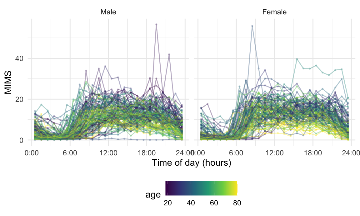
These data can be analyzed using hour-specific linear models that
regress bin-average MIMS values on age and
gender. This does not account for the temporal structure of
the diurnal profiles except through the binning that aggregates data.We
fit a standard linear model for with the average MIMS value between 1:00
and 2:00pm as a response by we unnesting the hour-level functional
observations and subset to the interval of current interest.
linear_fit =
  nhanes_df %>%
  select(SEQN, age, gender, MIMS_hour) %>%
  tf_unnest(MIMS_hour) %>%
  filter(MIMS_hour_arg == 13.5) %>%
  lm(MIMS_hour_value ~ age + gender, data = .)
Here is a table showing regression results.
| term | estimate | std.error | statistic | p.value |
|---|---|---|---|---|
| (Intercept) | 16.836 | 0.883 | 19.059 | 0.000 |
| age | -0.079 | 0.016 | -4.939 | 0.000 |
| genderFemale | 1.041 | 0.608 | 1.714 | 0.088 |
And here is a scatterplot illustrating the regression at this time point.
nhanes_df %>%
  select(SEQN, age, gender, MIMS_hour) %>%
  tf_unnest(MIMS_hour) %>%
  filter(MIMS_hour_arg == 13.5) %>%
  modelr::add_predictions(linear_fit) %>%
  ggplot(aes(x = age, y = MIMS_hour_value, color = gender)) +
  geom_point(alpha = .5, lwd = .9) +
  geom_line(aes(y = pred), linewidth = 1.1) +
      labs(x = "Age", y = "Hour Average MIMS")
## Warning in geom_point(alpha = 0.5, lwd = 0.9): Ignoring unknown parameters:
## `linewidth`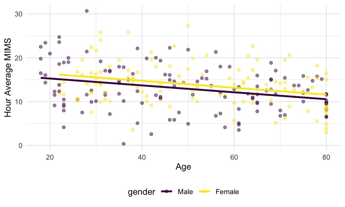
In this plot, the binned-average MIMS values decrease with age, and female participants may have somewhat higher values than male participants.
Associations between binned-average MIMS values and age
and gender will vary by hour. Next we unnest the
subject-specific functional observation and then re-nest within hour;
the result is a dataframe containing 24 rows, one for each hour, with a
column that contains a list of hour-specific dataframes containing the
MIMS_hour_value, age, and gender.
By mapping over the entries in this list, we can fit hour-specific
linear models and extract tidied results.
hourly_regressions =
  nhanes_df %>%
  select(SEQN, age, gender, MIMS_hour) %>%
  tf_unnest(MIMS_hour) %>%
  rename(hour = MIMS_hour_arg, MIMS = MIMS_hour_value) %>%
  nest(data = -hour) %>%
  mutate(
    model = map(.x = data, ~lm(MIMS ~ age + gender, data = .x)),
    result = map(model, broom::tidy)
  ) %>%
  select(hour, result)
We process these results obtain hourly confidence intervals and then
structure coefficient estimates and confidence bands as tf
objects. The result is a three-row dataframe, with rows for the
intercept, age, and gender effects; columns include the term name as
well as the coefficient estimates and the upper and lower limits of the
confidence bands.
hour_bin_coefs =
  hourly_regressions %>%
  unnest(cols = result) %>%
  rename(coef = estimate, se = std.error) %>%
  mutate(
    ub = coef + 1.96 * se,
    lb = coef - 1.96 * se
  ) %>%
  select(hour, term, coef, ub, lb) %>%
  tf_nest(coef:lb, .id = term, .arg = hour)
Because the coefficient estimates in coef are
tf objects, we can plot these using
geom_spaghetti in tidyfun; to
emphasize the estimates at each hour, we add points using
geom_meatballs. Confidence bands are shown by specifying
the upper and lower limits, and we facet by term to see each coefficient
separately.
hour_bin_coefs %>%
  ggplot(aes(y = coef, color = term)) +
  geom_spaghetti() +
  geom_meatballs() +
  geom_errorband(aes(ymax = ub, ymin = lb, fill = term)) +
  facet_wrap("term", scales = "free") +
  scale_x_continuous(
    breaks = seq(0, 24, length = 5),
    labels = str_c(seq(0, 24, length = 5), ":00")) +
  labs(x = "Time of day (hours)", y = "Coefficient")
The intercept shows a fairly typical diurnal pattern, with low activity in the night and higher activity in the day. After adjusting for age, women are somewhat less active in the middle of the night but more active during the daytime hours. Meanwhile, after adjusting for gender, older participants are generally less active at all times.
The hour-level analysis is an informative exploratory approach, but has several limitations. Most obviously, it aggregates data within prespecified bins, and in doing so loses some of the richness of the underlying data. That aggregation induces some smoothness by relying on the underlying temporal structure, but this smoothness is implicit and dependent on the bins that are chosen. To emphasize these points, we can repeat the bin-level analysis using 1-minute epochs.
min_regressions =
  nhanes_df %>%
  select(SEQN, age, gender, MIMS_tf) %>%
  tf_unnest(MIMS_tf) %>%
  rename(epoch = MIMS_tf_arg, MIMS = MIMS_tf_value) %>%
  nest(data = -epoch) %>%
  mutate(
    model = map(.x = data, ~lm(MIMS ~ age + gender, data = .x)),
    result = map(model, broom::tidy)
  ) %>%
  select(epoch, result) %>%
  unnest(result)

min_regressions =
  min_regressions %>%
  rename(coef = estimate, se = std.error) %>%
  mutate(
    ub = coef + 1.96 * se,
    lb = coef - 1.96 * se
  ) %>%
  select(epoch, term, coef, ub, lb) %>%
  tf_nest(coef:lb, .id = term, .arg = epoch) %>%
  mutate(method = "Pointwise") %>%
  relocate(method)
Results for one-minute epochs are in the next figure.
min_regressions %>%
  ggplot(aes(y = coef, color = term)) +
  geom_spaghetti() +
  geom_meatballs() +
  geom_errorband(aes(ymax = ub, ymin = lb, fill = term)) +
  facet_wrap("term", scales = "free") +
  scale_x_continuous(
    breaks = seq(0, 24, length = 5),
    labels = str_c(seq(0, 24, length = 5), ":00")) +
  labs(x = "Time of day (hours)", y = "Coefficient")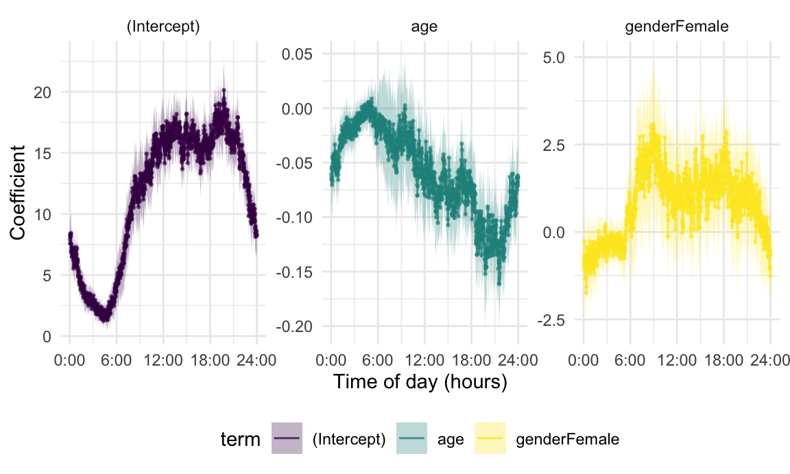
The qualitative results and their interpretations are similar – the intercept suggests a usual circadian rhythm, and the age indicates that activity generally decreases with increasing age, and the gender effect shows that female participants were more active than male participants. But this also shows some difficulties inherent in binning-based analyses. These do not leverage the temporal structure directly in the estimation process. A correct approach to inference is not obvious, both because of the need for some degree of smoothness across time and also because within-subject residuals will have a temporal correlation structure. A more subtle issue is that we implicitly rely on curves being observed over the same grid, or at least that a rolling mean is a plausible way to generate binned averages, and this approach may not work when data are sparse or irregular across subjects.
Solutions to these problems are the goal of various approaches to function-on-scalar regression, which seeks to explicitly model coefficients in a way that induces smoothness; in some way accounts for within-curve correlation; and extends to a variety of data generating scenarios.
Linear Function-on-Scalar Regression
Let \(y_i:\mathcal{S}\rightarrow \mathbb{R}\) be a functional response of interest for each study participant, \(i=1,\ldots,n\), and \(x_{i1}\) and \(x_{i2}\) be two scalar predictors. In the example on this page, the functional response is the MIMS profile for each participant, and the scalar predictors of interest are age in years and a variable indicating whether participant \(i\) is male (\(x_{i2} = 0\)) or female (\(x_{i2} = 1\)). The linear function-on-scalar regression for this setting is \[E[Y_i(s)] = \beta_0(s) + \beta_1(s) x_{i1} + \beta_2(s) x_{i2}\] with coefficients \(\beta_q:\mathcal{S}\rightarrow \mathbb{R}\), \(q \in \{0, 1, 2\}\) that are functions measured over the same domain as the response. Scalar covariates in this model can exhibit the same degree of complexity as in non-functional regressions, allowing any number of continuous and categorical predictors of interest.
Coefficient functions encode the varying association between the response and predictors, and are interpretable in ways that parallel non-functional regression models. In particular, \(\beta_0(s)\) is the expected response for \(x_{i1} = x_{i2} = 0\); \(\beta_1(s)\) is the expected change in the response for each one unit change in \(x_{i1}\) while holding \(x_{i2}\) constant; and so on. These are often interpreted at specific values of \(s \in \mathcal{S}\) to gain intuition for the associations of interest. Residuals in this model will contain deviations between the observed responses and the expected values based on the linear predictor.
The linear FoSR model has several advantages. Because coefficients are functions observed on \(\mathcal{S}\), they can be estimated using techniques that explicitly allow for smoothness across the functional domain. This smoothness, along with appropriate error correlation structures, provides an avenue for correct statistical inference. Considering coefficients as functions also opens the door to data generating mechanisms for observed data that would be challenging or impossible in more exploratory settings, such as responses that are observed on grids that are sparse or irregular across subjects.
Estimation of Fixed Effects
Functional responses are observed over a discrete grid \(\mathbf{s} = \{s_1, ..., s_J\}\) which, for now, we will assume to be common across subjects so that for subject \(i\) the observed data vector is \(\mathbf{y}_i^{T} = [y_i(s_1), ..., y_i(s_J)]\). From the FoSR, we have \[E[\mathbf{y}_i^{T}] = \mathbf{x}_i \begin{bmatrix} \beta_{0}(s_1) & ... & \beta_{0}(s_J)\\ \beta_{1}(s_1) & ... & \beta_{2}(s_J)\\ \beta_{2}(s_1) & ... & \beta_{3}(s_J) \end{bmatrix} \] where \(\mathbf{x}_i = [1, x_{i1}, x_{i2}]\) is the row vector containing scalar terms that defines the regression model. This expression is useful because it connects a \(1 \times J\) response vector to a recognizable row in a standard regression design matrix and the matrix of functional coefficients.
Estimation of coefficients will rely on approaches that have been used elsewhere with nuances specific to the FoSR setting. As a starting point, we will expand each \(\beta_q(s) = \sum_{k=1}^K\beta_{qk} B_k(s)\) using the basis \(B_1(s),\ldots,B_K(s)\). While many choices are possible, we will use a spline expansion. Using this, the \(3 \times J\) matrix of coefficient functions can be expressed using \[ \begin{bmatrix} \beta_{11} & \beta_{21} & \beta_{31}\\ \vdots & \vdots & \vdots \\ \beta_{1K} & \beta_{2K} & \beta_{3K} \end{bmatrix} \begin{bmatrix} \boldsymbol{B}_{1}(s_1) & ... & \boldsymbol{B}_{K}(s_1)\\ \vdots & & \vdots \\ \boldsymbol{B}_{1}(s_J) & ... & \boldsymbol{B}_{K}(s_J) \end{bmatrix}. \]
Conveniently, one can concisely combine and rewrite the previous expressions. Let \(\boldsymbol{B}(s_{j}) = [B_1(s_{j}), \ldots, B_K(s_{j})]\) be the \(1 \times K\) row vector containing the basis functions evaluated at \(s_{j}\) and \(\boldsymbol{B}(\mathbf{s})\) be the \(K \times J\) matrix containing basis functions evaluated over the grid \(\mathbf{s}\). Further, let \(\mathbf{\beta}_{q} = [\beta_{q1}, \ldots, \beta_{qK}]^{T}\) be the \(K \times 1\) vector of basis coefficients for function \(p\) and \(\boldsymbol{\beta} = [\mathbf{\beta}^{T}_{0}, \mathbf{\beta}^{T}_{1}, \mathbf{\beta}^{T}_{2}]^{T}\) be the \((3 \cdot K) \times 1\) vector constructed by stacking the vectors of basis coefficients. For the \(J \times 1\) response vector \(\mathbf{y}_i\), we have \[ E[\mathbf{y}_i] = [\mathbf{x}_i \otimes \boldsymbol{B}(\mathbf{s})] \boldsymbol{\beta} \] where \(\otimes\) is the Kronecker product.
This expression for a single subject can be directly extended to all subjects. Let \(\mathbf{y}\) be the \((n \cdot J) \times 1\) vector created by stacking the vectors \(\mathbf{y}_i\) and \(\boldsymbol{X}\) be \(n \times 3\) matrix created by stacking the vectors \(\mathbf{x}_i\). Then \[ E[\mathbf{y}] = [\boldsymbol{X} \otimes \boldsymbol{B}(\mathbf{s})] \boldsymbol{\beta}. \] This formulation, while somewhat confusing at first, underlies many implementations of the linear FoSR model. First, we note that the matrix \(\boldsymbol{X}\) is the design matrix familiar from non-functional regression models, and includes a row for each subject and a column for each predictor. The Kronecker product with the basis \(\boldsymbol{B}(\mathbf{s})\) replicates that basis once for each coefficient function; this product also ensures that each coefficient function, evaluated over \(\mathbf{s}\), is multiplied by the subject-specific covariate vector \(\mathbf{x}_i\). Finally, considering \([\boldsymbol{B}(\mathbf{s}) \otimes \boldsymbol{X}]\) as the full FoSR design matrix and \(\boldsymbol{\beta}\) as a vector of coefficients to be estimated explicitly connects the FoSR model to standard regression techniques.
Estimation using ordinary least squares
Estimation the spline coefficients helps to build intuition for the
inner workings of more complex estimation strategies. We will regress
the daily MIMS data on age and gender to illustrate this approach.
Recall that nhanes_df stores MIMS as a
tf vector; some of the code below relies on extracting
information from a tf object.
For this model, the code chunk below defines the standard design
matrix \(\boldsymbol{X}\) and the
response vector \(\mathbf{y}\). The
call to model.matrix() uses a formula that correctly
specifies the predictors, and obtaining the response vector
y unnests the tf vector and then extracts the
observed responses for each subject.
X_des =
  model.matrix(
    SEQN ~ gender + age,
    data = nhanes_df
  )

y =
  nhanes_df %>%
  tf_unnest(MIMS_tf) %>%
  pull(MIMS_tf_value)
The next code chunk constructs the spline basis matrix \(\boldsymbol{B}(\mathbf{s})\) and the
Kronecker product \([\boldsymbol{B}(\mathbf{s}) \otimes
\boldsymbol{X}]\). The spline basis is evaluated over the grid
\(\mathbf{s}\) pulled from
MIMS, and uses \(K = 30\)
basis functions.
epoch_arg = seq(1/60, 24, length = 1440)

basis =
  splines::bs(epoch_arg, df = 30, intercept = TRUE)

X_kron_B = kronecker(X_des, basis)
Using these, the direct application of usual formulas provides OLS
estimates of the spline coefficients. Reconstructing coefficient
functions is possible, and the results can be converted to a
tf vector for plotting and manipulation. The code chunk
below estimates spline coefficients.
spline_coefs = solve(t(X_kron_B) %*% X_kron_B) %*% t(X_kron_B) %*% yWe now construct, organize, and plot coefficient functions.
OLS_coef_df =
  tibble(
    method = "OLS",
    term = colnames(X_des),
    coef =
      tfd(
        t(basis %*% matrix(spline_coefs, nrow = 30)),
        arg = epoch_arg)
  )

OLS_coef_df %>%
  ggplot(aes(y = coef, color = term)) +
  geom_spaghetti(lwd = 1.1, alpha = .75) +
  facet_wrap("term", scales = "free") +
  scale_x_continuous(
    breaks = seq(0, 24, length = 5),
    labels = str_c(seq(0, 24, length = 5), ":00")) +
  labs(x = "Time of day (hours)", y = "Coefficient")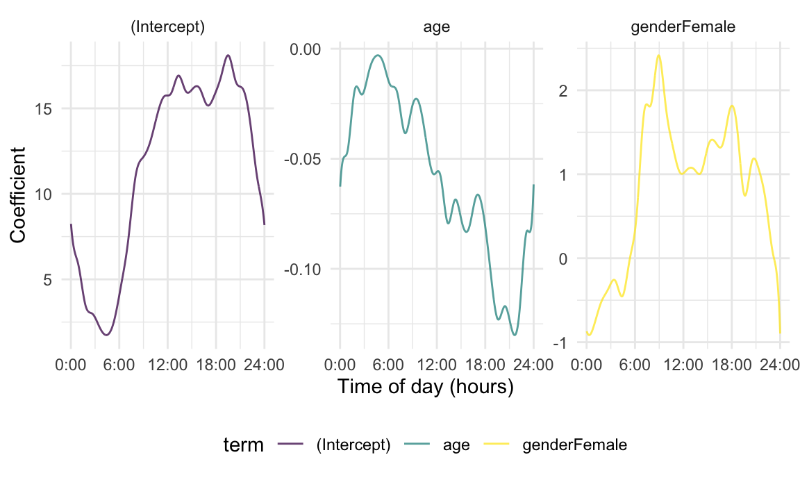
Comparing these results to those obtained from epoch-specific regressions begins to indicate the benefits of a functional perspective. We will next incorporate smoothness penalties and account for complex error correlations, but it is helpful to view these as variations on a familiar regression framework.
Estimation using smoothness penalties
Spline expansions for coefficient functions in the linear FoSR model makes the functional nature of the observed data and the model parameters explicit, and distinguishes this approach from multivariate or epoch-based alternatives. However, using a spline expansion introduces questions about how best to balance flexibility with goodness-of-fit. It is common to use a large value for \(K\) and introduce smoothness-enforcing penalties to prevent overfitting.
Solutions obtained using OLS also arise using maximum likelihood estimation. Assume that residuals \(\mathbf{\epsilon}_i^{T} = [\epsilon_i(s_1), ..., \epsilon_i(s_J)]\) observed on \(\mathbf{s}\) are \(\mathrm{iid}\) are drawn from a mean-zero normal distribution with variance \(\sigma^{2}_{\epsilon}\) that is constant over time points \(\mathbf{s}\) and subjects \(i\). Maximizing the (log) likelihood \(\mathcal{L}(\boldsymbol{\beta}; \mathbf{y})\) induced by this assumption with respect to spline coefficients is equivalent to the OLS approach. We can add penalties \(P\left[\beta_{q}(s) \right]\) to enforce smoothness in estimates of coefficient functions; a common choice is the second derivative penalty \(\int_{\mathcal{S}} \left[\beta_{q}^{''}(s) \right]^2 ds\). The second derivative penalty and many others can be expressed in terms of the corresponding coefficient vector, resulting in the penalized likelihood \[ \mathcal{L}(\boldsymbol{\beta}; \mathbf{y}) + \sum_{q} \lambda_{q} P\left[\mathbf{\beta}_{q} \right]\] where tuning parameters \(\lambda_{q}\) control the balance between goodness-of-fit and complexity of the coefficient functions \(\beta_{q}(s)\).
Here we are emphasizing a penalized likelihood approach rather than using the penalized residual sum of squares. Focusing on the penalized likelihood makes the extension to non-continuous response functions (e.g. binary rest-active trajectories instead of MIMS profiles) relatively direct by changing the assumed outcome distribution, and will similarly facilitate modeling and including error correlation structures. More importantly, it is possible to view the likelihood-based framework as a variation on mixed-model approaches to penalized spline smooth smoothing emphasized throughout the book, and which underlies many FoSR implementations.
We will use the gam function in the well-developed
mgcv package to fit the FoSR model with smoothness
penalties. First, we explicitly create the binary indicator variable for
gender, and organize data into “long” format by unnesting
the MIMS data stored as a tf object. The resulting
dataframe has a row for each subject and epoch, containing the
MIMS outcome in that epoch as well as the scalar covariates
of interest. This is analogous to the creation of the response vector
for model fitting using OLS, and begins to organize covariates for
inclusion in a design matrix.
nhanes_for_gam =
  nhanes_df %>%
  mutate(gender = as.numeric(gender == "Female")) %>%
  tf_unnest(MIMS_tf) %>%
  rename(epoch = MIMS_tf_arg, MIMS = MIMS_tf_value)
With data in this form, we can fit the FoSR model using
mgcv::gam() as follows.
gam_fit =
  gam(MIMS ~ s(epoch) + s(epoch, by = gender) + s(epoch, by = age),
      data = nhanes_for_gam)
Conceptually, this specification indicates that each observed
MIMS value is the combination of three smooth functions of
epoch: an intercept function, and the products of
coefficient functions and scalar covariates gender and
age. Specifically, the first model term
s(epoch) indicates the evaluation of a spline expansion
over values contained in the epoch column of the data frame
nhanes_for_gam. The second and third terms add
by = gender and by = age, respectively, which
also indicate spline expansions over the epoch column but
multiply the result by the corresponding scalar covariates. This process
is analogous to the creation of the design matrix \([\boldsymbol{B}(\mathbf{s}) \otimes
\boldsymbol{X}]\), although gam()’s function
s() allows users to flexibly specify additional options for
each basis expansion.
In contrast to parameter estimation using OLS, smoothness is induced
in parameter estimates through explicit penalization. By default,
gam() uses thin-plate splines with second derivative
penalties, and selects tuning parameters for each coefficient using GCV
or REML.
The results contained in gam_fit are not directly
comparable to those we’ve seen elsewhere, and extracting coefficient
functions requires some additional work. The predict.gam()
function can be used to return each element of the linear predictor for
a provided data frame. In this case, we hope to return smooth functions
of epoch corresponding to the intercept and coefficient
functions. We therefore create a data frame containing an
epoch column consisting of the unique evaluation points of
the observed functions (i.e. minutes); a column gender, set
to 1 for all epochs; and a column age, also
set to 1 for all epochs.
gam_pred_obj =
  tibble(
    epoch = epoch_arg,
    gender = 1,
    age = 1,
  ) %>%
  predict(gam_fit, newdata = ., type = "terms")
The result contained in gam_pred_obj is a
1440 x 3 matrix, with columns corresponding to \(\beta_0(\mathbf{s})\), \(1 \cdot \beta_1(\mathbf{s})\), and \(1 \cdot \beta_2(\mathbf{s})\). We convert
these to tfd objects in the code below. Note that
gam() includes the overall intercept as a (scalar) fixed
effect, which must be added to the intercept function.
gam_coef_df =
  tibble(
    method = "GAM",
    term = c("(Intercept)", "genderFemale", "age"),
    coef =
      tfd(t(gam_pred_obj), arg = epoch_arg)) %>%
  mutate(coef = coef + c(coef(gam_fit)[1], 0, 0))
With data structured in this way, we can then plot coefficient functions using tools seen previously.
gam_coef_df %>%
  ggplot(aes(y = coef, color = term)) +
  geom_spaghetti(lwd = 1.1, alpha = .75) +
  facet_wrap(vars(term), scales = "free") +
  scale_x_continuous(
    breaks = seq(0, 24, length = 5),
    labels = str_c(seq(0, 24, length = 5), ":00")) +
  labs(x = "Time of day (hours)", y = "Coefficient")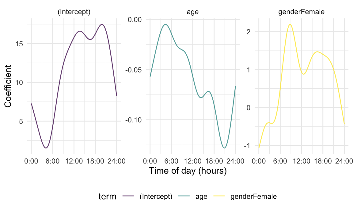
The plot below includes estimates obtained from the three approaches
seen so far, and facilitates a comparison of methods. Each approach –
separate epoch-level regressions, FoSR using OLS to estimate spline
coefficients, and FoSR implemented with smoothness penalties in
mgcv::gam() – yields qualitatively similar results
regarding the effect of age and gender on diurnal MIMS trajectories.
This suggests that all approaches can be used at least in exploratory
analyses or to understand general patterns. That said, there are obvious
differences. The epoch-level regressions do not borrow information
across adjacent time points, and the OLS is sensitive to dimension of
the basis expansion in the model specification; both are wigglier, and
perhaps less plausible, than the method that includes smoothness
penalties. As a result, methods that explicitly borrow information
across time and implement smoothness penalties with data-driven tuning
parameters are often preferred for formal analyses.
ggplot(mapping = aes(y = coef, color = method)) +
  geom_spaghetti(data = min_regressions, alpha = .5) +
  geom_spaghetti(data = OLS_coef_df, linewidth = 1.2) +
  geom_spaghetti(data = gam_coef_df, linewidth = 1.2) +
  facet_wrap(vars(term), scales = "free") +
  scale_x_continuous(
    breaks = seq(0, 24, length = 5),
    labels = str_c(seq(0, 24, length = 5), ":00")) +
  labs(x = "Time of day (hours)", y = "Coefficient")
Accounting for Error Correlation
To this point, we have developed tools for estimating coefficient functions while setting aside concerns about residual correlation. Of course, in most FoSR settings residuals are indeed correlated; in our example, MIMS values at 10:00am are informative for values at 1:00pm.
Most methods focus on modeling the residuals \(\epsilon_i(s)=X_i(s)+e_i(s)\), where \(X_i(s)\) follows a mean zero Gaussian Process (GP) with covariance function \(\boldsymbol{\Sigma}\) and \(e_{i}(s)\) are independent \(N(0,\sigma^2_e)\) random errors. There are many strategies to model jointly the nonparametric mean and error structure of this model including: (1) joint modeling based on FPCA decomposition of \(X_i(s)\); (2) functional additive mixed models (FAMM) using spline expansions of the error term \(X_i(\cdot)\); and (3) Bayesian posterior simulations for either type of expansion.
Modeling residuals with FPCA and gam
Combining FoSR with FPCA for correlated residuals suggests the following model structure: \[Y_i(s) = \beta_0(s) + \beta_1(s) x_{i1} + \beta_2(s) x_{i2} + \sum_{k = 1}^{K} \xi_{ik}\phi_k(s) + e_{i}(s)\] \[\xi_{ik} \sim [0, \lambda_k]; \epsilon_i(s) \sim N[0, \sigma^2].\] As before, functions are observed over discrete values \(\mathbf{s}_i = \{s_1, ..., s_{J_i}\}\) that can be dense or sparse, regular or irregular, and shared across subjects or not.
Our approach to estimating coefficient functions \(\beta_0(s)\) will remain essentially unchanged. The challenge now is how best to estimate terms in the sum \(\sum_{k = 1}^{K} \xi_{ik}\phi_k(s)\), keeping in mind that both subject level scores \(\xi_{ik}\) and shared directions of variation \(\phi_k(s)\) are unknown. A key observation is that if the \(\phi_k(s)\) are known or if estimates \(\hat{\phi}_k(s)\) are available, then scores can be estimated as random effects in a mixed model. Our approach will be to obtain estimates of the \(\phi_k(s)\), so that coefficient functions \(\beta_{q}(s)\) and scores \(\xi_{ik}\) can be simultaneously estimated using penalized splines and random effects, respectively. Although it is not strictly necessary to fit and interpret the results of a FoSR model, recognizing that mixed models underlie the penalized spline estimation for coefficient functions as well as the random effects estimation for scores connects these two model components and facilitates implementation.
First, we will assume that \(K = 1\) and \(\phi_{1}(s) = 1\) for all \(s \in \mathcal{S}\) as an illustration. This effectively adds a subject-level random intercept to the FoSR model, and is a useful contrast between longitudinal data analysis and functional data analysis: the former typically makes assumptions that limit the flexibility of subject-level estimates over the observation interval \(\mathcal{S}\), while the latter uses data-driven approaches to add flexibility where appropriate.
To fit the random intercept model, we adapt our previous
implementation for penalized spline estimation in a number of ways.
Recall that nhanes_for_gam contains a long-form dataframe
with rows for each subject and epoch, and columns containing
MIMS and scalar covariates. This dataframe also contains a
column of subject IDs SEQN; importantly, this is encoded as
a factor variable and therefore can be used to define subjects in the
following a random effects specification. In the formula component of
the model below, the terms corresponding to fixed effects are unchanged,
but we add a term s(SEQN) with the argument
bs = "re". This creates a “smooth” term with a random
effects “basis” – essentially taking advantage of the noted connection
between semiparametric regression and random effects estimation to
obtain subject-level random effects estimates and the corresponding
variance component. Finally, we note that we use bam
instead of gam, and add arguments
method = "fREML" and discrete = TRUE. These
changes dramatically decrease computation times.
nhanes_gamm_ranint =
  nhanes_for_gam %>%
  bam(MIMS ~ s(epoch) + s(epoch, by = gender) + s(epoch, by = age) +
             s(SEQN, bs = "re"),
      method = "fREML", discrete = TRUE, data = .)
Next, we will use a two-step approach to model correlated residuals using FPCA. The first step is to fit a FoSR model assuming uncorrelated errors to obtain estimates of fixed effects \(\beta_{q}(s)\) and fitted values \(\hat{Y_i}(s)\) for each subject. From these, we compute residuals \(\hat{w}_i(s) = Y_{i}(s) - \hat{Y_i}(s)\) which can be decomposed using standard FPCA methods to produce estimates of FPCs \(\hat{\phi}_{k}(s)\). In the second step, the \(\hat{\phi}_{k}(s)\) are treated as “known”; coefficient functions \(\beta_{q}(s)\) and subject-level scores \(\xi_{ik}\) are then estimated simultaneously. The NHANES data are densely measured over a regular grid that is common to all subjects and we implement the FPCA step using the FACE method.
In the code below, we first construct a dataframe that contains
fitted values and residuals, and can subsequently be used as the basis
for FPCA. We start with nhanes_for_gam, and add fitted
values from our penalized spline estimation assuming independent errors
in gam_fit; residuals are created by subtracting the fitted
values from the MIMS observations. After keeping only the
subject ID SEQN, epoch and the residual values
for each subject at each epoch, we nest to create a dataframe in which
residual curves are tf values. Using this dataframe, we
conduct FPCA using the rfr_fpca() function in the
refundr R package. At the time of writing,
refundr is under active development and contains
reimplementations of many functions in the refund package
using tidyfun for data organization. By default, for data
observed over a regular grid rfr_fpca() uses FACE to
conduct FPCA. We specify two additional arguments in this call. First,
center == FALSE avoids recomputing the mean function since
we are using residuals from a previous fit. Second, we set the smoothing
parameter by hand using lambda = 50; this produces smoother
FPCs than the default implementation.
nhanes_fpca_df =
  nhanes_for_gam %>%
  mutate(
    fitted = fitted(gam_fit),
    resid = MIMS - fitted) %>%
  select(SEQN, epoch, resid) %>%
  tf_nest(resid, .id = SEQN, .arg = epoch)

nhanes_resid_fpca =
  rfr_fpca("resid", nhanes_fpca_df, center = FALSE, lambda = 50)
## Warning: domain for tfb_fpc can't be larger than observed arg-range -- extrapolating FPCs is a bad idea.
##  domain reset to [0.017,24]
The second step in our two-stage approach is to treat the resulting
FPCs as “known” so that scores can be estimated as random effects. We
will use a variation on the random intercept implementation to do this.
In particular, our goal remains to estimate a random effect or score
\(\xi_{ik}\) for each subject and FPC,
but now that score will multiply the FPC evaluated over the functional
domain. Put differently, we want to scale one component in our model by
another; to do this, we will again make use of the by
argument in the s() function.
The code chunk below defines the dataframe necessary to implement
this strategy. It repeats code seen before to convert the
nhanes_df dataframe to a format needed by
mgcv::gam(), by creating an indicator variable for
gender and unnesting the MIMS data stored as a
tf object. However, we also add a column fpc
that contains the first FPC estimated above. The FPC is the same for
each participant and here is treated as a tf object. We
then unnest both MIMS and fpc to produce a
long-format dataframe with row for each subject and epoch.
nhanes_for_gamm =
  nhanes_df %>%
  mutate(
    gender = as.numeric(gender == "Female"),
    fpc = tfd(nhanes_resid_fpca$efunctions[,1])) %>%
  tf_unnest(cols = c(MIMS_tf, fpc)) %>%
  rename(epoch = MIMS_tf_arg, MIMS = MIMS_tf_value, fpc = fpc_value) %>%
  select(-fpc_arg)
With these data organized appropriately, we can estimate coefficient
functions and subject-level FPC scores using a small modification to our
previous random intercept approach. We again estimate subject-level
effects using s(SEQN) and a random effect “basis” that adds
a random intercept for each participant. Including by = fpc
scales the random effect basis by the FPC value in each epoch,
effectively creating the term \(\xi_{i1}
\phi_{1}(s)\) by treating \(\phi_{1}(s)\) as known.
nhanes_gamm_fpc =
  nhanes_for_gamm %>%
  bam(MIMS ~ s(epoch, fx = T) + s(epoch, by = gender, fx = T) + s(epoch, by = age, fx = T) +
             s(SEQN, bs = "re", by = fpc),
      discrete = TRUE, method = "fREML", data = .)
This implementation of the FoSR model using FPCA to account for residual correlation has important strengths. Penalized spline estimation of fixed effects leverages information across adjacent time points and enforces smoothness, and residual correlation is accounted for in a flexible, data-driven way. Some additional refinements are possible, and may be useful in practice; these include the incorporation of several FPCs into a term of the form \(\sum_{k = 1}^{K} \xi_{ik}\phi_k(s)\) and iterating so that FPCs are derived from a model that has accounted for residual correlation in the estimation of fixed effects.
We now show how to extract the quantities necessary to conduct estimation and inference for coefficient function \(\beta_{q}(s)\). Our approach to constructing pointwise confidence intervals is based on the spline-based estimation approaches considered so far, as well as the assumption that spline coefficient estimates have an approximately multivariate Normal distribution. Treating tuning parameters as fixed, for any \(s \in S\) the variance of \(\widehat{\beta}_q(s)\) is given by \[\mbox{Var}\{\widehat{\beta}_q(s)\} = \mathbf{B}(s) \mbox{Var}(\widehat{\boldsymbol{\beta}}_q) \mathbf{B}(s)^{t}\;, \] where \(\widehat{\boldsymbol{\beta}}_q\) is the vector of estimated spline coefficients. From this, one can obtain standard errors and construct a confidence interval for \(\beta_q(s)\) using the assumption of normality. A critical component is the covariance of estimated spline coefficients \(\mbox{Var}(\boldsymbol{\widehat{\beta}}_q)\), which is heavily dependent on the modeling assumptions used to estimate spline coefficients. We have fit three FoSR models using penalized splines for coefficient functions, with different assumptions about residuals.
To extract coefficient functions and their standard errors from the
objects produced by mgcv::gam(), we again make use of the
predict() function. This function takes an input dataframe
that has all covariates used in the model; here we will use the first
1440 rows of the nhanes_for_gamm dataframe,
which has all epoch-level observations for a single subject. We set
gender and age to 1 as before, so terms
produced by predict() will correspond to coefficient
functions. When calling predict, we now set the argument
se.fit = TRUE, so that both terms and their standard errors
are returned.
nhanes_fpc_pred_obj =
  nhanes_for_gamm[1:1440,] %>%
  mutate(gender = 1, age = 1) %>%
  predict(
    nhanes_gamm_fpc, newdata = .,
    type = "terms", se.fit = TRUE)
The output of predict() requires some processing before
plotting. We construct coef_df to contain the relevant
output, again using steps that are similar to those seen previously: a
term variable is created and coefficients are extracted and
converted to tf objects, and the model’s overall intercept
is added to the intercept function. There are some important changes,
however. Because we set se.fit = TRUE the result contains
both coefficients and standard errors, and we extract these from the
fit and se.fit elements of the object returned
by predict, respectively. The model that uses FPCA to
account for residual correlation also includes a coefficient for
SEQN, and so we use only the first three terms in the
model. Finally, the code also includes a step to obtain upper and lower
bounds of a 95% pointwise confidence interval, constructed by adding and
subtracting 1.96 times the standard error to the estimate for each
coefficient.
coef_df =
  tibble(
    term = c("(Intercept)", "genderFemale", "age"),
    coef = tfd(t(nhanes_fpc_pred_obj$fit[,1:3]), arg = epoch_arg),
    se = tfd(t(nhanes_fpc_pred_obj$se.fit[,1:3]), arg = epoch_arg)) %>%
  mutate(coef = coef + c(coef(nhanes_gamm_fpc)[1], 0, 0)) %>%
  mutate(
    ub = coef + 1.96 * se,
    lb = coef - 1.96 * se)
The same approach can be used to extract coefficient functions and
confidence intervals for the three approaches to accounting for residual
correlation. We implement this in the code chunk below, using the helper
function fosr_gam_res_to_tfd()
to process the gam() results for several fits by mapping
over a list of gam objects.
df =
  nhanes_for_gamm[1:1440,] %>%
  mutate(gender = 1, age = 1)

comparison_plot_df =
  tibble(
    method = c("Independent", "Random Intercept", "FPCA"),
    fit = list(gam_fit, nhanes_gamm_ranint, nhanes_gamm_fpc)
  ) %>%
  mutate(coefs = map(fit, fosr_gam_res_to_tfd, df = df)) %>%
  select(method, coefs) %>%
  unnest(coefs) %>%
  mutate(
    ub = coef + 1.96 * se,
    lb = coef - 1.96 * se) %>%
  mutate(
    method = fct_inorder(method)
  )
The results are combined into comparison_plot_df and
plotted in the figure below. Note the use of
geom_errorband(), which adds shaded regions according to
each coefficient functions upper and lower confidence limits.
comparison_plot_df %>%
  ggplot(aes(y = coef, color = term)) +
  geom_spaghetti() +
  geom_errorband(aes(ymax = ub, ymin = lb, fill = term)) +
  facet_grid(term ~ method, scales = "free") +
  scale_x_continuous(
    breaks = seq(0, 24, length = 5),
    labels = str_c(seq(0, 24, length = 5), ":00")) +
  labs(x = "Time of day (hours)", y = "Coefficient")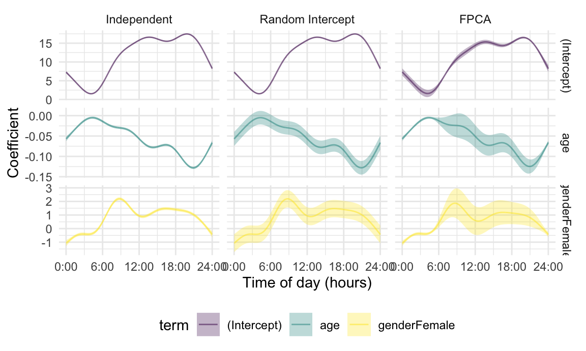
The coefficient functions obtained by all methods are similar to each other and to those based on epoch-level regressions. The confidence bands, meanwhile, differ substantially in a way that is intuitive based on the assumed error structures. Assuming independence fails to capture any of the correlation that exists within subjects, and therefore has overly narrow confidence bands. Using a random intercept accounts for some of the true correlation but makes restrictive parametric assumptions on the correlation structure. Because this approach effectively induces uniform correlation over the domain, the resulting intervals are wider than those of under the model assuming independence but have a roughly fixed width over the day. Finally, modeling residual curves using FPCA produces intervals that are narrower in the nighttime and wider in the daytime, which more accurately reflects the variability across subjects in this dataset. This model suggests a significant decrease in MIMS as age increases over much of the day, and a significant increase in MIMS comparing women to men in the morning and afternoon.
In some ways, it is unsurprising that the coefficient function
estimates produced under different assumptions are similar. After all,
each is an unbiased estimator for the fixed effects in the model. But
the complexity of the underlying maximization problem can produce
counter-intuitive results in some cases. In this analysis, the results
of the FPCA model fitting are sensitive to the degree of smoothness in
the FPC. When the less-smooth FPCs produced by the default FACE settings
were used, the coefficient function estimates were somewhat attenuated.
At the same time, the random effects containing FPC scores were
dependent on the scalar covariates in a way that exactly offset this
attenuation. This does not appear to be an issue with the
gam() implementation, because “by hand” model fitting
showed the same sensitivity to smoothness in the FPCs. Instead, we
believe this issues stems from subtle identifiability issues and the
underlying complexity of the penalized likelihood.
Modeling residuals using splines
A powerful approach to implementing FoSR is to model both the fixed
effects parameters \(\beta_q(s)\) and
the structured random residuals using penalized splines. This approach
has several advantages as it: (1) uses a pre-specified basis, which
avoids the potential problems associated with the uncertainty of FPCA
bases that are estimated from the data; (2) avoids the problem of
estimating an FPCA basis, which is especially useful when dealing with
non-Gaussian functions; (3) can be implemented in existing software; see
the refund::pffr(); (4) allows joint analysis of the model
using a fully specified, explicit likelihood; and (5) is consistent with
inferential tools for estimation, testing, and uncertainty
quantification.
We now show how to use refund::pffr() to fit the FoSR
model. For computational efficiency, we aggregate minute-level data into
hour-length bins and reduce each MIMS profile from 1440 to 24
observations. This step is achieved using the same code introduced to
implement binned regression. The hour-level MIMS is named
MIMS_hour_mat and stored as a matrix in a column, and we
emphasize that this data structure used is different from the data
structure used in the mgcv::bam() function, where
functional responses were organized in long format. Note that, as in the
gam fits, we explicitly create a binary indicator for the
gender variable.
nhanes_famm_df <-
  nhanes_df %>%
  mutate(
    gender = as.numeric(gender == "Female"),
    MIMS_hour_tf =
      tf_smooth(MIMS_tf, method = "rollmean", k = 60, align = "center"),
    MIMS_hour_tf = tfd(MIMS_hour_tf, arg = seq(.5, 23.5, by = 1))) %>%
  tf_unnest(MIMS_hour_tf) %>%
  rename(epoch = MIMS_hour_tf_arg, MIMS_hour = MIMS_hour_tf_value) %>%
  pivot_wider(names_from = epoch, values_from = MIMS_hour)
## setting fill = 'extend' for start/end values.
## Warning: There was 1 warning in `mutate()`.
## ℹ In argument: `MIMS_hour_tf = tf_smooth(MIMS_tf, method = "rollmean", k = 60,
##   align = "center")`.
## Caused by warning:
## ! non-equidistant arg-values in 'MIMS_tf' ignored by rollmean.

MIMS_hour_mat <-
  nhanes_famm_df %>%
  select(as.character(seq(0.5, 23.5, by = 1))) %>%
  as.matrix()

nhanes_famm_df <-
  nhanes_famm_df %>%
  select(SEQN, gender, age) %>%
  mutate(MIMS_hour_mat = I(MIMS_hour_mat))
We now fit the function-on-scalar model using pffr() to
analyze the association between age and gender on physical activity,
where each residual is modeled using penalized splines.
nhanes_famm =
  nhanes_famm_df %>%
  pffr(MIMS_hour_mat ~ age + gender + s(SEQN, bs = "re"),
       data = ., algorithm = "bam", discrete = TRUE,
       bs.yindex = list(bs = "ps", k = 15, m = c(2, 1)))
The fitted model is stored as the object nhanes_famm. To
visualize the fixed effects estimates and confidence bands, we use a
similar approach to the one that extracted estimates and SE from
mgcv objects, which is facilitated through the helper
function pffrcoef_to_tf(). Note
we again add the population intercept to the intercept function.
pffr_coef_df =
  tibble(
    term = c("(Intercept)", "age", "genderFemale"),
    raw_coef = coef(nhanes_famm)$smterms[1:3]
  ) %>%
  mutate(
    raw_coef = map(raw_coef, "coef"),
    coef = map(raw_coef, pffrcoef_to_tf)
  ) %>%
  select(term, coef) %>%
  unnest(coef) %>%
  mutate(
    coef = coef + c(nhanes_famm$coef[1], 0, 0),
    ub = coef + 1.96 * se,
    lb = coef - 1.96 * se)
## using seWithMean for  s(yindex.vec) .
The next Figure shows the fixed effects estimates obtained using
pffr(). Notice that these estimates are similar to those
using separate epoch-level regressions, and in particular those using
similar hour-level data. An advantage of this joint modeling approach is
that it gives smoother estimates and accounts for error
correlations.
pffr_coef_df %>%
  ggplot(aes(y = coef, color = term)) +
  geom_spaghetti() +
  geom_errorband(aes(ymax = ub, ymin = lb, fill = term))  +
  facet_wrap(~term, scales = "free") +
  scale_x_continuous(breaks = seq(0, 24, length = 5)) +
  labs(x = "Time of day (hours)", y = "Average MIMS") +
  scale_x_continuous(
    breaks = seq(0, 24, length = 5),
    labels = str_c(seq(0, 24, length = 5), ":00")) +
  labs(x = "Time of day (hours)", y = "Coefficient")
## Scale for x is already present.
## Adding another scale for x, which will replace the existing scale.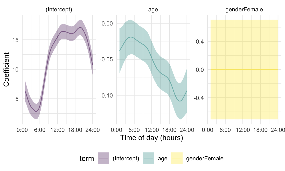
A scalable approach based on epoch-level regressions
FoSR modeling often involves high-dimensional data with resulting
computational pressures. In regressing MIMS values on
age and gender, we have largely avoided a
discussion of these issues by focusing on a subset comprised of 250
subjects. However, it is worth noting the scale of required matrix
computations. For 250 subjects observed over 1440 epochs each, design
matrices will have 360,000 rows; if 30 spline basis functions are used
in the estimation of coefficient functions, this design matrix will have
90 columns. Increasing the number of subjects or predictors will
exacerbate problems of scale. The tools we’ve used so far, in particular
the mgcv package for penalized spline estimate, are
well-developed and computationally efficient, but can nonetheless
struggle to meet the demands of some modern datasets.
A very simple alternative strategy revisits the epoch-level regressions that previously motivated a switch to “functional” techniques. Recall that the epoch-level regression models did not account for temporal structure, but simply fit standard regression models at each epoch separately. The “functional” approach explicitly accounted for temporal structure by expanding coefficient functions of interest and shifting focus to the estimation of spline coefficients. Instead, one can smooth epoch-level regression coefficients to obtain estimates of coefficient functions. Computationally, this requires fitting many simple models rather than one large model, and can scale easily as the number of subjects or covariates increases.
In Section RegBinData, we saw results of minute-level regression. The
code below implements that analysis, and is similar to the approach seen
for one-hour epochs. In particular, we unnest the MIMS
column containing a tf vector for functional observations,
which produces a long-format dataframe containing all subject- and
epoch-level observations. We then re-nest by epoch, so that
data across all subjects within an epoch are consolidated; this step
allows the epoch-by-epoch regressions of MIMS on
age and gender by mapping across epoch-level
datasets. The results of the regressions are turned into dataframes by
mapping the broom::tidy function across model results.
Finally, epoch-level regression results are unnested so that the
intercept and two regression coefficients are available for each
epoch.
min_regressions =
  nhanes_df %>%
  select(SEQN, age, gender, MIMS_tf) %>%
  tf_unnest(MIMS_tf) %>%
  rename(epoch = MIMS_tf_arg, MIMS = MIMS_tf_value) %>%
  nest(data = -epoch) %>%
  mutate(
    model = map(.x = data, ~lm(MIMS ~ age + gender, data = .x)),
    result = map(model, broom::tidy)
  ) %>%
  select(epoch, result) %>%
  unnest(result)
The next step in this analysis is to smooth the regression
coefficients across epochs. Many techniques are available for this; the
approach implemented below organizes epoch-level regression coefficients
as tf objects in the a term called coef, and
then smooths the results using a lowess smoother in the
tf_smooth() function. The resulting data frame has three
columns: term (taking values (Intercept),
age and genderFemale, coef
(containing the unsmoothed results of epoch-level regressions),
smooth_coef (containing the smoothed versions of values in
coef).
fui_coef_df =
  min_regressions %>%
  select(epoch, term, coef = estimate) %>%
  tf_nest(coef, .id = term, .arg = epoch) %>%
  mutate(smooth_coef = tf_smooth(coef, method = "lowess"))
The figure below contains a panel for each term, and shows epoch-level and smooth coefficients. Note the similarity between the smoothed coefficients and those obtained by “functional” approaches, including penalized splines; this suggests that this technique is a plausible and scalable approach to FoSR modeling.
fui_coef_df %>%
  ggplot(aes(y = smooth_coef, color = term)) +
  geom_spaghetti(lwd = 1.2) +
  geom_spaghetti(aes(y = coef), alpha = .2)  +
  facet_wrap(~term, scales = "free") +
  scale_x_continuous(
    breaks = seq(0, 24, length = 5),
    labels = str_c(seq(0, 24, length = 5), ":00")) +
  labs(x = "Time of day (hours)", y = "Coefficient")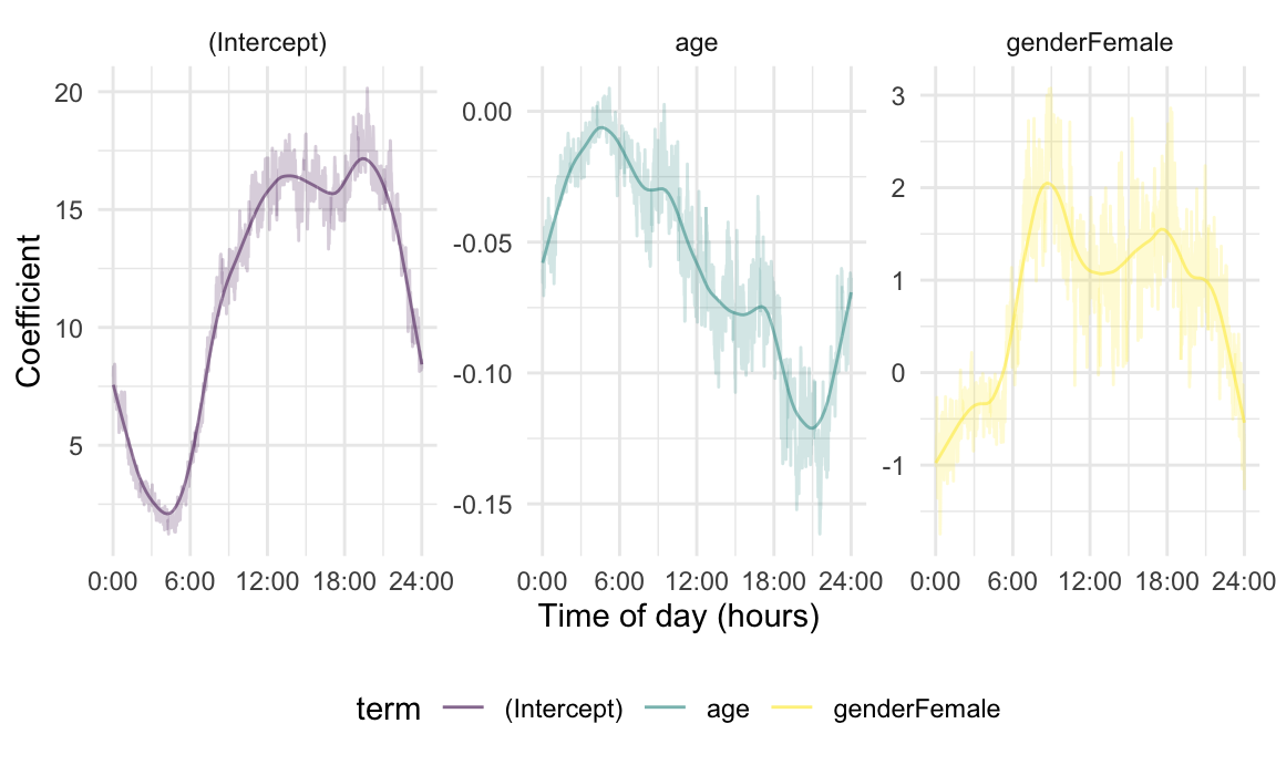
An important focus is to model error structures and thereby obtain accurate inference. The scalable approach we suggest in this section models each epoch separately, but the residual correlation is implicit: regression coefficients across epochs are related through the residual covariance. This fact, and the scalability of the estimation algorithm, suggests that bootstrapping is a plausible inferential strategy in this setting. In particular, we suggest to: resample participants, including full response functions, with replacement to create bootstrap samples; fit epoch-level regressions for each bootstrap sample and smooth the results; and construct confidence intervals based on the results. This resampling strategy preserves the within-subject correlation structure of the full data without making additional assumptions on the form of that structure. From a computational perspective, bootstrap always increases computation time because one needs to refit the same model multiple times. However, pointwise regression and smoothing is a simple and relatively fast procedure, which makes the entire process much more computationally scalable than joint modeling . Moreover, the approach is easy to parallelize which can further improve computational times.
Our implementation of this analysis relies on a helper function nhanes_boot_fui(), which has
arguments seed and df. This function contains
the following steps: first, it sets the seed to ensure reproducibility
and then creates a bootstrap sample from the provided dataframe; second,
it creates the hat matrix that is shared across all epoch-level
regressions; third, it estimates epoch-level coefficients by multiplying
the hat matrix by the response vector at each epoch; and fourth, it
smooths these coefficients and returns the results.
The code chunk below obtains results across 250 bootstrap samples. In practice one may need to run more bootstrap iterations, but this suffices for illustration. After unnesting, we have smooth coefficients for each iteration.
fui_bootstrap_results =
  tibble(iteration = 1:250) %>%
  mutate(
    boot_res = map(iteration, nhanes_boot_fui, df = nhanes_df)
  ) %>%
  unnest(boot_res)
The next shows results of this analysis. We include the full-sample estimates and estimates obtained in 25 bootstrap samples in the background. We also show pointwise confidence intervals by adding and subtracting \(1.96\) times the pointwise standard errors obtained via the bootstrap to the full-sample estimates. Constructing joint confidence intervals requires one to account for the complete joint distribution of the functions.
fui_bootstrap_results %>%
  group_by(term) %>%
  summarize(
    est = mean(smooth_coef),
    se = sd(smooth_coef)) %>%
  mutate(
    ub = est + 1.96 * se,
    lb = est - 1.96 * se) %>%
  ggplot(aes(y = est, color = term)) +
  geom_spaghetti(lwd = 1.2, alpha = .9) +
  geom_spaghetti(
    data = filter(fui_bootstrap_results, iteration <= 25),
    aes(y = smooth_coef), alpha = .25, lwd = .5) +
  geom_errorband(aes(ymax = ub, ymin = lb, fill = term), alpha = .15)  +
  facet_wrap(~term, scales = "free")  +
  scale_x_continuous(
    breaks = seq(0, 24, length = 5),
    labels = str_c(seq(0, 24, length = 5), ":00")) +
  labs(x = "Time of day (hours)", y = "Coefficient")